In our previous post, we introduced the setup of predictive modeling in chip manufacturing and operations, highlighting common challenges such as imbalanced datasets and the need for more nuanced evaluation metrics. We also explored how NVIDIA CUDA-X data science libraries—like cuDF and cuML—can help overcome these challenges and accelerate machine learning workflows.In this blog, we shift focus to the next critical step: feature engineering. We have observed that carefully crafted features—built efficiently with GPU acceleration—can significantly improve both model performance and deployment readiness.For example, since our models often need to execute and relay predictions within tight 15-minute factory windows, using CUDA-X Data Science libraries and the feature engineering techniques discussed below has enabled us to reduce ETL processing time by up to 40% while maintaining or improving model accuracy. This efficiency directly impacts operational viability in high-throughput manufacturing environments. We focus here on three key techniques:
- Leveraging positional features
- Coalescing test results
- Incorporating prior probabilities based on historical context
All of these transformations are designed to run at scale on NVIDIA GPUs using cuDF, which brings zero code change acceleration to pandas pipelines using the cudf.pandas interface.
Leveraging positional features: spatial context matters
In semiconductor manufacturing, the physical location of a chip on a wafer can significantly influence its performance. Defects or anomalies often exhibit spatial patterns, making positional data invaluable for predictive modeling. By incorporating features like X and Y coordinates of a die on a wafer, as well as the Z-position (representing the wafer’s sequence in a lot), we can capture these spatial dependencies.
To enrich our models with this spatial context, we calculate metrics such as the average yield of neighboring units. This involves identifying adjacent dies and computing statistics like mean yield or defect rates within a defined neighborhood. By using cuDF’s GPU-accelerated operations, we can perform these computations efficiently, even on large datasets.
import cudf.pandas as pd# Assume 'df' is a cuDF DataFrame with columns: 'wafer_id', 'x', 'y', 'yield'df = pd.DataFrame({ 'wafer_id': [...], 'x': [...], 'y': [...], 'yield': [...]})# Create shifted neighbors and join themfor dx, dy in [(-1,0), (1,0), (0,-1), (0,1)]: neighbor = df.copy() neighbor['x'] += dx neighbor['y'] += dy df = df.merge(neighbor[['wafer_id', 'x', 'y', 'yield']], on=['wafer_id', 'x', 'y'], how='left', suffixes=('', f'_n{dx}{dy}'))# Average neighbor yieldsneighbor_cols = [col for col in df.columns if 'yield_n' in col]df['neighbor_yield'] = df[neighbor_cols].mean(axis=1) |
These pipelines are deployed in environments where thousands of chips are being tested daily. GPU acceleration ensures these neighborhood-based transformations run efficiently even under strict production SLAs—sometimes requiring model inference and ETL within a ten-minute factory window.
Coalescing test results: synthesizing multiple measurements
Chips undergo various tests during manufacturing, often resulting in multiple measurements for the same parameter under different conditions, like voltage or temperature. To create a unified feature from these disparate readings, we employ a technique called coalescing. This process involves grouping related test results and computing a representative statistic, such as the mean or maximum value.
Using cudf.pandas, we can perform these operations efficiently:
# Assume 'df' has columns: 'chip_id', 'test_name', 'voltage', 'time', 'measurement'# Filter tests for a specific voltagedf_filtered = df[df['voltage'] == 1.0]# Sort by time to get the latest measurementdf_sorted = df_filtered.sort_values(['chip_id', 'test_name', 'time'], ascending=[True, True, False])# Drop duplicates to keep the latest measurement per chipdf_latest = df_sorted.drop_duplicates(subset=['chip_id', 'test_name'])# Compute the mean measurement per chipdf_coalesced = df_latest.groupby(['chip_id'])['measurement'].mean().reset_index(name='coalesced_measurement') |
This approach ensures that each chip is represented by a single, consolidated measurement, enhancing the quality of the input features for our models. In fact, applying this coalescing step has improved model accuracy in some of our projects and contributed to a 20% reduction in unnecessary tests—directly impacting production costs and cycle time.
Incorporating prior probabilities: learning from historical context
Historical data can provide valuable insights into the likelihood of certain outcomes. By calculating prior probabilities based on factors like the tester’s ID, wafer position in lot, die coordinates on the wafer, or other contextual information, we can inform our models about inherent biases or tendencies in the manufacturing process.
For example, if certain testers historically yield higher failure rates, incorporating this information can improve predictive accuracy.Another common example is that chips closer to the edge of the wafer have a higher or lower pass rate than average.
Here’s how we can compute prior probabilities using cuDF:
# Assume 'df' has columns: 'ECID', 'tester_id', 'XY_coord', pass_fail' (1 for pass, 0 for fail). ECID refers to Exclusive Chip ID.# Prior pass rates per tester and (x,y) coordinates of chiptester_pass_prob = df.groupby('tester_id')['pass_fail'].mean().reset_index(name='prior_pass_rate_tester')chipxy_pass_prob = df.groupby('XY_coord')['pass_fail'].mean().reset_index(name='prior_pass_rate_XY')# Merge back to the original DataFramedf = df.merge(tester_pass_prob, on='tester_id', how='left')df = df.merge(chipxy_pass_prob, on='XY_coord'', how='left') |
By adding these prior probabilities as features, we provide our models with a nuanced understanding of the manufacturing environment’s historical performance. Since this computation is performed daily across large volumes of test data, the ability to perform these ‘groupby’ and ‘join’ operations on the GPU helps us stay within the narrow ETL windows we often face—especially in late-stage testing where results must be acted on quickly.
Conclusion
Feature engineering in operations is about both boosting accuracy and ensuring that insights arrive fast enough to drive decisions within operational timelines. With CUDA-X GPU-accelerated libraries, we’ve built feature engineering pipelines that can infer in less than 10 minutes and grow across thousands of units daily. This process used to take 20–25 minutes on CPU-based ETL pipelines under similar workloads. This acceleration enables us to meet tight SLAs for test operations without sacrificing feature complexity.. Whether it’s spatial smoothing, signal coalescing, or historical priors, each of these techniques has played a role in boosting our yield insights and reducing test redundancy in production.
For more information on CUDA-X Data Science libraries:
To test drive cuML, try this ‘Getting Started’ notebook in Colab with a free GPU runtime enabled, and for an introduction to cuML zero code change, you can read about our recent launch in this blog. To learn more about how you can leverage CUDA-X libraries that require no API code changes, check out the courses in our DLI Learning Path for accelerated data science.